Replication Exercise

In this exercise we show the validity of the package in replicating Phillips et al. (2015).

We download the CAPE data from the Shiller website to perform the exercise.

import pandas as pd

url: str = (
    "https://img1.wsimg.com/blobby/go/e5e77e0b-59d1-44d9-ab25-4763ac982e53/downloads/02d69a38-97f2-45f8-941d-4e4c5b50dea7/ie_data.xls?ver=1743773003799"
)

data: pd.DataFrame = (
    pd.read_excel(
        url,
        sheet_name="Data",
        skiprows=7,
        usecols=["Date", "P", "D", "E", "CAPE"],
        skipfooter=1,
        dtype={"Date": str, "P": float},
    )
    .rename(
        {
            "P": "sp500",
            "CAPE": "cape",
            "Date": "date",
            "D": "dividends",
            "E": "earnings",
        },
        axis=1,
    )
    .assign(
        date=lambda x: pd.to_datetime(x["date"].str.ljust(7, "0"), format="%Y.%m"),
    )
    .set_index("date", drop=True)
)

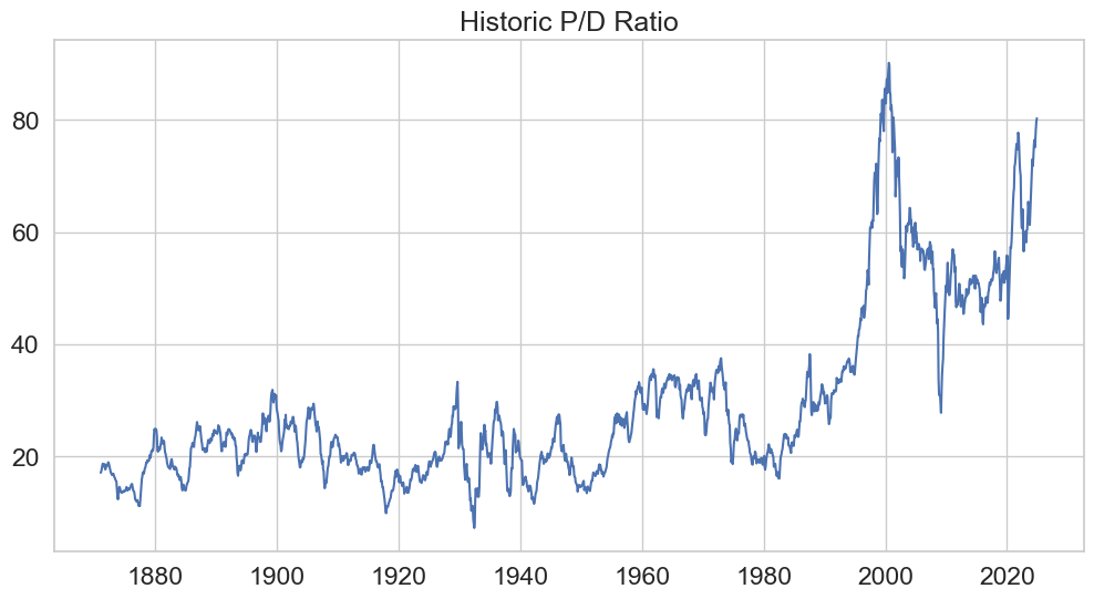
We look for the existence of bubbles in the Price-Dividend ratio.

pdratio: pd.Series = data["sp500"] / data["dividends"]
pdratio = pdratio.dropna()

import matplotlib.pyplot as plt
import seaborn as sns

sns.set_theme(
    context="notebook",
    style="whitegrid",
    font_scale=1.5,
    rc={"figure.figsize": (12, 6)},
)

plt.plot(pdratio)
plt.title("Historic P/D Ratio")
plt.show()

Using the psytest package, we first initialize the object using the PSYBubbles function.

from psytest import PSYBubbles
from numpy import datetime64

psy: PSYBubbles[datetime64] = PSYBubbles.from_pandas(
    data=pdratio, minwindow=None, lagmax=0, minlength=None
)

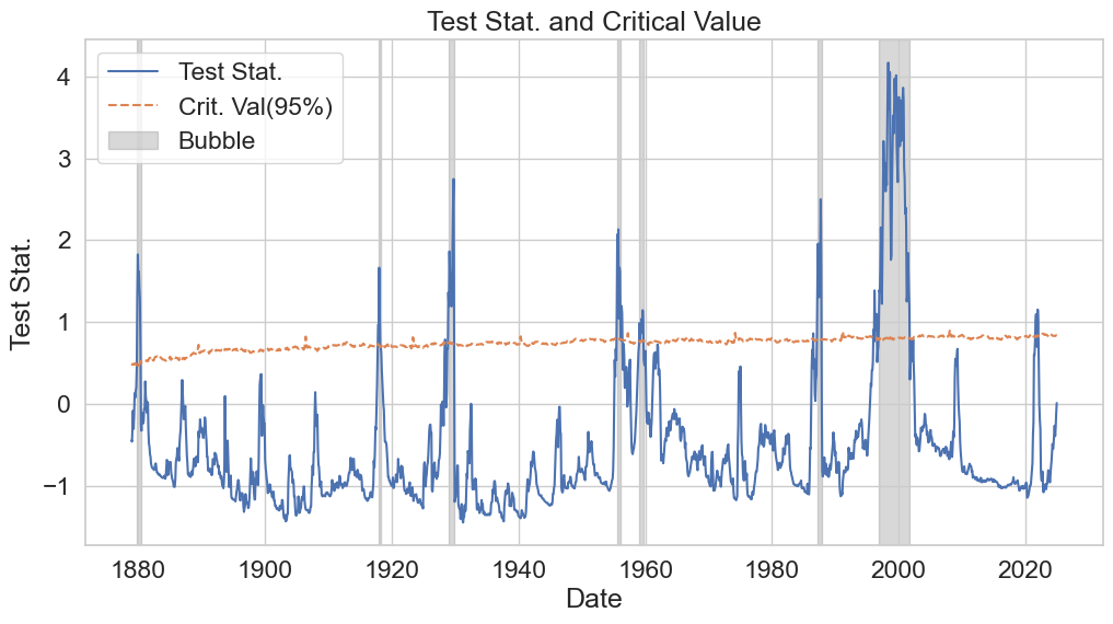
Then we calculate the test statistics and critical values. We will be using a significance level of 5% using the available tabulated data by setting fast=True.

stat: dict[datetime64, float] = psy.teststat()
cval: dict[datetime64, float] = psy.critval(alpha=0.05, fast=True)

Using these objects, we find the occurances of bubbles in the data:

bubbles: list[tuple[datetime64, datetime64 | None]] = psy.find_bubbles(alpha=0.05)

plt.plot(stat.keys(), stat.values(), label="Test Stat.")
plt.plot(cval.keys(), cval.values(), linestyle="--", label="Crit. Val(95%)")
for i, bubble in enumerate(bubbles):
    plt.axvspan(
        bubble[0],
        bubble[1] if bubble[1] is not None else pdratio.index[-1],
        color="gray",
        alpha=0.3,
        zorder=-1,
        label="Bubble" if i == 0 else None,
    )
plt.legend()
plt.title("Test Stat. and Critical Value")
plt.xlabel("Date")
plt.ylabel("Test Stat.")
plt.show()

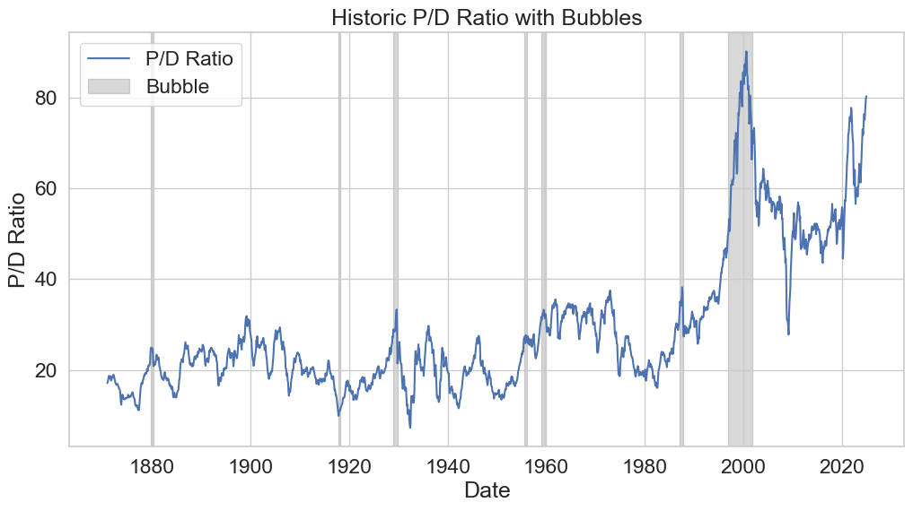
plt.plot(pdratio, label="P/D Ratio")
for i, bubble in enumerate(bubbles):
    plt.axvspan(
        bubble[0],
        bubble[1] if bubble[1] is not None else pdratio.index[-1],
        color="gray",
        alpha=0.3,
        zorder=-1,
        label="Bubble" if i == 0 else None,
    )
plt.legend()
plt.title("Historic P/D Ratio with Bubbles")
plt.xlabel("Date")
plt.ylabel("P/D Ratio")
plt.show()

bubbles_table: pd.DataFrame = pd.DataFrame(bubbles, columns=["start", "end"]).assign(
    duration=lambda x: x["end"] - x["start"],
)
bubbles_table

	start	end	duration
0	1879-11-01	1880-06-01	213 days
1	1917-11-01	1918-05-01	181 days
2	1929-01-01	1929-11-01	304 days
3	1955-07-01	1956-03-01	244 days
4	1959-02-01	1959-10-01	242 days
5	1987-02-01	1987-11-01	273 days
6	1996-11-01	2001-10-01	1795 days

Which match with the ones on the original paper (p.p. 1066).